Semantic Search at Scale: How We Transformed Product Retrieval at Joko
Let’s imagine you have an AI agent acting as your personal shopping assistant. You would want to talk to it the same way you would to a human: “I’m looking for a minimalist beige coat for fall, not too expensive” or “something that goes with my long red dress”.
From the user’s point of view, this feels straightforward. From a retrieval standpoint, it isn’t. These requests combine intent, constraints, and style preferences in a way that doesn’t match cleanly with product titles or structured attributes. Traditional keyword-based retrieval engines struggle with this: they often miss context, synonyms, and style preferences, and they treat “something that goes with my long red dress” as just another bag of words.
At Joko, this challenge lies at the core of building Joko AI, our intelligent shopping assistant, which operates on a continuously updated catalog of over 200 million products from thousands of merchants. This system must handle complex natural-language queries, ensure fast and accurate retrieval, and maintain interactive response times, all while operating on our massive catalog of products.
In this article, we focus on one foundational question: how do you retrieve the right products at scale, fast, when user queries are vague, conversational, and stylistic?
We’ll walk through why classical keyword-based search pipelines fall short at this scale, how semantic (vector-based) search changes the retrieval paradigm, and what trade-offs emerge when moving from a prototype to a system that must serve millions of real users. We’ll also introduce a minimal semantic search proof of concept you can run yourself, designed to isolate the core retrieval mechanics without the complexity of full conversational systems.
🗝️ Why keyword search isn’t enough
At Joko AI’s core lies a product catalog with hundreds of millions of items from thousands of merchants. Its engine must understand natural-language shopping queries and return relevant results from this catalog almost instantly.
Earlier versions of our search method relied on a classical keyword-based pipeline. A query like “I’m looking for a minimalist beige coat for fall” would first be decomposed into explicit terms (e.g., “beige”, “coat”), and structured constraints (such as a price range). These signals were then used to query a full-text search engine to retrieve candidate products, apply filters, and re-rank results. Several steps in the pipeline relied on LLM calls, some executed in parallel to keep end-to-end latency within acceptable bounds.
This approach performs reasonably well when users type short, literal queries that match product metadata (e.g., “black Levi’s jeans”). However, it quickly shows its limits as queries become conversational or intent-heavy. Synonyms, paraphrases, and style-driven requests (e.g., “a minimalist beige coat for fall”) are hard to capture with plain keywords, especially when the catalog descriptions themselves are sparse, noisy, or inconsistent. The system must also juggle with multilingual input, brand names, and structured attributes such as sizes or categories, further complicating retrieval.
In practice, making a keyword-based system work for natural-language shopping queries requires far more than a single query against a search index. To approximate user intent, the system must first generate multiple query variants in advance: expanding each term with synonyms and paraphrases, mapping words to several potential product categories, and handling multilingual or stylistic expressions that do not appear verbatim in product metadata. Each of these variants is executed separately, often across different fields or indices, producing large candidate sets that must then be aggressively filtered and re-ranked to remove irrelevant results. Because keyword matching is inherently brittle, many retrieved products only partially match the user’s request, forcing additional post-processing steps to restore relevance.
When the results are still unsatisfactory, a feedback loop is required: the initial query must be rewritten, constraints adjusted, and the whole process repeated. This accumulation of query generation, execution, filtering, re-ranking, and iterative refinement quickly turns a “simple” keyword search into a multi-stage workflow with high latency, making it difficult to maintain fast, interactive response times at scale.
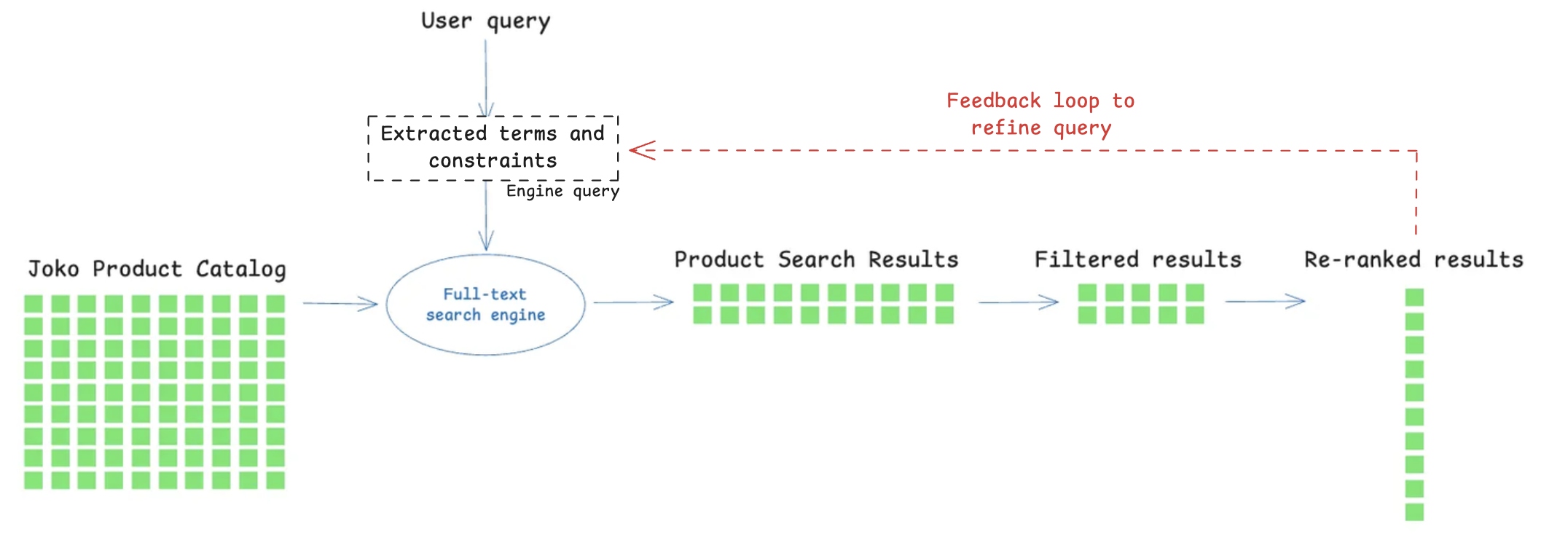
Figure 1: A simple keyword-based pipeline
We therefore needed a retrieval paradigm that could reason more directly about user intent. This is where semantic search came in.
🏹 Here come the vectors: what semantic search brings
Semantic search replaces keyword matching with dense vector representations of both queries and products. Instead of asking “does this word appear in the title?”, we encode each text into a high-dimensional vector and look for products whose vectors are closest to the query in that space. In other words, close meanings will end up close in the vector space, even if the exact words differ.
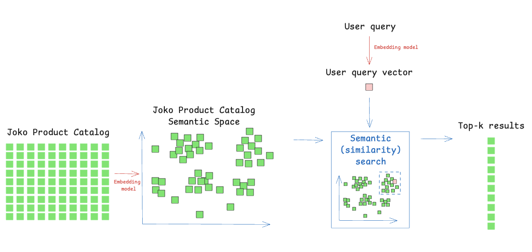
Figure 2: A classic semantic search pipeline
More importantly, semantic search changes what “matching” actually means. Instead of requiring that user terms explicitly appear in product titles or descriptions, it captures meaning. Synonyms, paraphrases, style-related intent, and multilingual phrasing are all naturally handled by the embedding model, which is something keyword search fundamentally struggles with, especially on noisy or incomplete catalog data. This makes vector search a powerful foundation for intent understanding, while keyword search remains a surgical tool for exact constraints like specific brands, sizes, or price filters. Combined in an approach called Hybrid Search, the two methods complement each other: semantic search retrieves products that match the intent and style of the query, while keyword search enforces hard constraints like brands, sizes, or price ranges. This lets us return results that align with both what users mean and what they explicitly require.
✨ How semantic search changed product retrieval at Joko
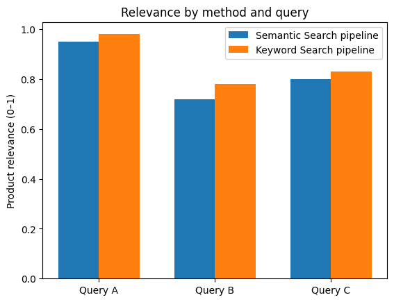
To evaluate whether changes to a retrieval method have a meaningful impact on product discovery, we base our analysis on the measurement of retrieval relevance. Retrieval relevance reflects the system’s ability to return products that satisfy the user’s intent for a given query, and therefore serves as the primary indicator of search quality.
In our evaluation framework, relevance judgments are given using a large language model (LLM) acting as an automated evaluator within an LLM-as-a-judge framework. For each query–product pair, the model is prompted to determine whether the retrieved product satisfies the user’s query intent. This approach provides a scalable and cost-efficient alternative to manual annotation while maintaining as much consistency across evaluations as possible.
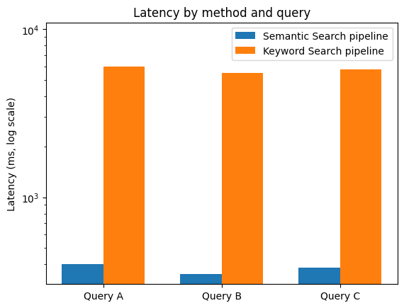
Based on this evaluation method, the semantic search framework managed to achieve comparable retrieval relevance as our previous keyword-based system while reducing end-to-end latency from several seconds to under 500ms for typical queries.
Why is semantic search faster at equal relevance? This speed-up is not accidental: it comes from a fundamental simplification to the retrieval process. To reach a comparable level of relevance with a keyword-based approach, the system must compensate for the lack of semantic understanding through a lot of effort. A single user query typically fans out into many keyword queries: terms are expanded with synonyms, mapped to multiple possible categories, translated or normalized, and executed across several product fields. Because keyword matching is permissive, these queries often retrieve large and noisy candidate sets, which then require heavy filtering and re-ranking to eliminate irrelevant results. When relevance is still insufficient, a feedback loop kicks in: the query is rewritten, constraints are relaxed or tightened, and the whole pipeline is executed again. Each of these steps adds latency, complexity, and operational fragility.
Semantic search short-circuits this entire process. A single embedding captures most of the user’s intent (style, context, and meaning included) and retrieves a compact, high-quality candidate set in one nearest-neighbor lookup. Instead of compensating for weak matching with multiple queries and post-processing stages, relevance is baked directly into the retrieval step. The result is a much shorter execution path: fewer queries, fewer filters, no iterative refinement loop, and therefore far lower end-to-end latency.
In other words, semantic search is not faster because it is more optimized, it is faster because it removes entire layers of work that keyword-based systems need in order to approximate relevance at scale.
The following figures show retrieval results for selected anonymized queries.
🔭 A minimal semantic search PoC you can run at home
Rather than starting with hundreds of millions of products, we would like to introduce semantic search through a small, reproducible example that you can run in a notebook.
In this example, we use the Joko Clothing Products dataset. It’s a dataset of 17k products of clothing items for which we limited the information to the product title and description.
This experiment has three parts:
-
Download the Joko Clothing Products dataset from Kaggle
Download the dataset on this link and create your Python notebook.
You can now load the dataset as a pandas dataframe with the following code.
# !pip install pandas # Uncomment inside a fresh notebook import pandas as pd # Load the Joko Clothing Products dataset dataset df = pd.read_csv("joko_products.csv") # Concatenate title + description into a single text field df["text"] = ( df["originalTitle"].fillna("") + " " + df["longDescription"].fillna("") ).str.strip()Note: To keep this example simple, we only use the title and description columns, concatenating them to create a single text field for encoding.
-
Embedding the dataset
For this example, we decided to use an OpenAI embedding model,
text-embedding-3-largebut you can pick any modern text embedding model, including open-source ones. We embed the data in batches.# !pip install openai numpy # Uncomment inside a fresh notebook import numpy as np from tqdm import tqdm from openai import OpenAI # Set an OpenAI API key here OPENAI_API_KEY = "..." client = OpenAI(api_key=OPENAI_API_KEY) # Define an embedding model EMBEDDING_MODEL = "text-embedding-3-large" def embed_batch(texts): """ Compute embeddings for a list of texts. Returns a list of embedding vectors (lists of floats). """ response = client.embeddings.create( input=texts, model=EMBEDDING_MODEL, ) return [item.embedding for item in response.data] # Embed the whole catalog in small batches batch_size = 256 all_embeddings = [] for start in tqdm(range(0, len(df), batch_size)): end = start + batch_size batch_texts = df["text"].iloc[start:end].tolist() batch_embeddings = embed_batch(batch_texts) all_embeddings.extend(batch_embeddings) # Convert to a NumPy array for future indexing embeddings = np.array(all_embeddings, dtype="float32") df["embedding"] = list(embeddings) -
Indexation and semantic search
For indexation and semantic search that can be run locally on most computers, a classic library to use is FAISS (Facebook AI Similarity Search). FAISS is a library for fast similarity search over embeddings. It enables scalable nearest-neighbor retrieval.
FAISS gives us fast nearest-neighbor search over the embedding space. Because both products and queries are normalized and compared via inner product (equivalent to cosine similarity after L2-normalization), “closeness” now means “semantic similarity” rather than “shares the same keywords”.
For a first PoC, an in-memory FAISS index is well-suited: you feed it the product vectors, and it returns the top-k nearest neighbors for any query vector.
A simple search loop then becomes:
- embed the user query,
- ask the index for the k-closest products,
- display the corresponding items.
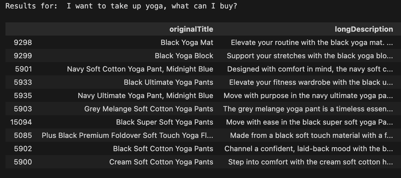
#!pip install faiss-cpu  # Uncomment inside a fresh notebook
import faiss

# We’ll use cosine similarity by normalizing vectors and using an inner-product index
dim = embeddings.shape[1]
faiss.normalize_L2(embeddings)

index = faiss.IndexFlatIP(dim)  # IP = inner product
index.add(embeddings)

print("Number of vectors in index:", index.ntotal)

def embed_query(query):
    """Embed and normalize a single query string."""
    vec = np.array(embed_batch([query])[0], dtype="float32")
    vec = vec.reshape(1, -1)
    faiss.normalize_L2(vec)
    return vec

def search(query, k = 5):
    """
    Runs a semantic search over the products.
    Returns a small dataframe with the top-k matching products.
    """
    q_vec = embed_query(query)
    scores, indices = index.search(q_vec, k)

    # Flatten the results and select matching rows
    idx = indices[0]
    results = df.iloc[idx][["originalTitle", "longDescription"]].copy()
    results["score"] = scores[0]
    return results

# Example queries
query = "I want to take up yoga, what can I buy?"
print("Results for: ", query)
display(search(query, k=10))
💪🏻 Now you can check out the results!
For example, for “I want to take up yoga, what can I buy?” we get the following results:
Try these other queries to see the true power of semantic search in action:
- “Ripped jeans with strass”
- “Clothes for summer”
- “Outfit for attending a wedding”
- “Sports clothes for running”
⇒ Even with a basic semantic search pipeline and no pre- or post-processing, the results are highly relevant to these semantically rich queries like they never would have been with keyword-based retrieval in the same conditions. Disclaimer: They are however not always perfect with such a simple workflow!
🎢 Hands-on for scale: building a Qdrant-backed vector search PoC
Now you know how vector search works at a small scale, but what about searching efficiently across tens or hundreds of millions of products? That’s where specialized vector databases like Qdrant come in. Qdrant is a cloud-native vector database built around HNSW approximate nearest-neighbor search, designed specifically for this purpose.
The approach is the same as what you’ve experienced at a small scale: they encode products and queries into vectors. But the storage, indexing, and scaling are handled for you, easily tunable and optimized for larger product catalogs.
💚 This Qdrant PoC is intentionally small and self-contained, but it mirrors the key ingredients of a production-grade semantic search backend.
The Qdrant PoC using the Joko Clothing Products dataset includes the following steps:
-
Prepare your data and embeddings
You can reuse the product dataset from the minimal PoC. Embed the product dataset the same way it was described in the last PoC, or save and reuse the embeddings generated before. You now have access to the texts and their corresponding embeddings in the same dataframe
df.texts = (df["originalTitle"] + " -- " + df["longDescription"]).tolist() vectors = [v.tolist() if hasattr(v, "tolist") else v for v in df["embedding"]] -
Create a collection in Qdrant
Create a Qdrant account on their website and create a free cluster. They will provide you with a corresponding URL and API key.
The following code aims to help you define a collection with the right vector size and distance metric (e.g., cosine). Qdrant builds an HNSW index under the hood, with tunable parameters to trade off between latency, recall, and memory.
from qdrant_client import QdrantClient, models

qdrant_client = QdrantClient(
    url="...", # Your cluster URL
    api_key="...") # Your API key

collection_name = "products-with-openai-large" ## Name Example

DIM = 3072  # for OpenAI text-embedding-3-large

qdrant_client.create_collection(
    collection_name=collection_name,
    vectors_config=models.VectorParams(size=DIM, distance=models.Distance.COSINE))
You can access the collections in your notebook with the following line:
print(qdrant_client.get_collections()) -
Ingest and query
You can now upload your vectors in batches.
from qdrant_client.models import PointStruct

# Prepare points for insertion
points = []
for i, (text, vector) in enumerate(zip(texts, vectors)):
    # Create payload with metadata
    payload = {
        "original_title": df.iloc[i]["originalTitle"],
        "long_description": df.iloc[i]["longDescription"],
        # Add any other metadata from your DataFrame
        # "additional_field": df.iloc[i]["additional_field"],
    }

    # Create point
    point = PointStruct(
        id=df.index[i],  # Generate unique ID
        vector=vector,
        payload=payload
    )
    points.append(point)

# Insert points into collection
# For large datasets, insert in batches
batch_size = 100
for i in range(0, len(points), batch_size):
    batch = points[i:i + batch_size]
    qdrant_client.upsert(
        collection_name=collection_name,
        points=batch
    )
At query time, you:
- embed the user’s text,
- send a “search” request to Qdrant asking for the top-k closest vectors,
- optionally filter on metadata (e.g., category = “sneakers”, price < X),
- render the products corresponding to the returned IDs.
def search_qdrant(query_text, limit=10):
    # Step 1: Embed the query text using OpenAI (same model you used for indexing)
    response = openai_client.embeddings.create(
        model="text-embedding-3-large", # Define your embedding model
        input=query_text
    )
    query_vector = response.data[0].embedding

    # Step 2: Search Qdrant using the query vector
    start_time = time.time()
    results = qdrant_client.search(
        collection_name=collection_name, # Define your collection name
        query_vector=query_vector,
        limit=limit
    )
    end_time = time.time()
    latency = end_time - start_time

    I = [[result.id for result in results]]

    for index_nb in I[0]:  # I[0] contains the indices
        print(df.iloc[index_nb]['originalTitle'])

# Example queries
query = "I want to take up yoga, what can I buy?"
print("Results for: ", query)
search_qdrant(query)
⇒ For identical queries on the Joko Clothing Products dataset, Qdrant consistently delivers similar relevance with significantly lower latency, up to roughly 3× to 11× faster, thanks to its optimized HNSW implementation and cloud infrastructure.
🚀 Beyond this post: what it takes to build an AI shopping agent
We hope this article gave you a clear and concrete view of what vector search brings to large-scale product retrieval, and why it has become such a powerful tool for modern search systems.
That said, vector search is only one ingredient in what it takes to build a truly useful AI shopping assistant. Helping users navigate hundreds of millions of products is an inherently hard problem. Real-world shopping queries are vague, contextual, and often underspecified, and solving them reliably requires more than a single retrieval technique.
At Joko AI, product discovery relies on advanced agentic workflows that orchestrate multiple tools: semantic and keyword search, structured filters, ranking models, business constraints, web searches, and iterative reasoning steps. Vector search plays a central role in understanding intent and narrowing the search space, but it is most effective when combined with other components that refine, validate, and contextualize results.
This journey, from exploratory notebooks to production systems serving real users, is the kind of work we do every day at Joko. If you’re curious to learn more or simply enjoy discussing large-scale search, retrieval, and AI systems, feel free to reach out. We’re always happy to talk about our engineering challenges.
And if you want to help us build this next generation of shopping experiences, we’re hiring in France and Spain 👉 https://www.welcometothejungle.com/en/companies/joko/jobs 👋